Cahill 1909
Cahill-Keyes 1975
|
Cahill 1909
|
Go back to
Gene Keyes home page
Cahill-Keyes 1975 |
| Cahill-Keyes Octant Graticule:
Principles and Specifications with Perl programs and OpenOffice.org 2.0 macros for 1/1,000,000 Megamap Gene Keyes 2010-08-20
©1975, 1980, 2010 by Gene Keyes
For fair use, with source credit, by anyone: copy, share, adapt, whatever. (Optional: send me your link!) For commercial use, contact gene.keyes~~at~~gmail~~dot~~com Abstract
Notes on Re-designing B.J.S. Cahill's Butterfly World Map Critique of Dymaxion Map as compared to Cahill's Notes on Scaling Cahill and Cahill-Keyes Maps Photos of the Cahill-Keyes Megamap Prototypes Geocells and the Megamap 10 Principles for a Coherent World Map System B.J.S. Cahill Resource Page |
| Contents
|
| 1) Fundamental considerations
We now get into what Cahill called the "intensive mathematical
details", which must fulfill my four essential design criteria
for the Cahill-Keyes master map:1) Visual fidelity to a globe in each and all of its eight equal octants, as well as showing each and all of its 64,800 one-degree geocells (except for the sliver-like 3,600 at the poles between 90 and 85°, drawn with 1° latitudes, but 5° longitudes );
Those design criteria in turn imposed some constraints, and indicate why the map is done in a certain way, and not some other way. (Cahill himself had evolved at least five different projection variations within his basic framework, but for reasons explained elsewhere, I started from scratch on a different path.) Besides the four main criteria stated above, three other considerations had to be met; again, differing in detail from Cahill: 5) That the octants be entirely symmetrical: all six end segments be equal to each other, and all three main mid-segments likewise equal one another.My design had to simultaneously satisfy all seven desiderata, none of which were present in Cahill's versions. It is their combination which establishes the character of the Cahill-Keyes — and entailed such difficulty in doing it. As Cahill himself wrote, "simplicity in most things is achieved by a circuitous route through all manner of complications." (1912, p. 164) ____________ 2) X-Y coordinates by hand or
computer
From 1980 to 1984, I computed all the x-y coordinates of all 8,100 geocells of an entire Cahill-Keyes Octant Graticule (minus the 450 polar spiky ones, drawn @ 1 x 5°), copying the 5-decimal-place numbers by hand into tables, from a TI-30 scientific calculator, and doing others with a BASIC program into a fanfold printout. This was well before the Internet. Now that I have revived this project for my website, after a 25-year dormancy, I boggled at keyboarding so much data. However, my companion Mary Jo Graça has patiently written a Perl program (p. 2 below) to re-calculate all those x-y coordinates and output them in HTML tables here (p. 3). Next, she exerted her coding skills to prepare macros (p. 4 and 5) using the Perl data, which could plot the map graticule via a vector drawing program. In doing these digital versions, I have been the architect, as it were, and Mary Jo the engineer. At first we were using an outdated 1993 Mac version of TurboCAD, but its exported .dxf files proved unusable, and it could not do very large scales. So we switched to OpenOffice.org Draw 2.0 (OOo for short; it is cross-platform, and free.). Though more difficult for Mary Jo to program its macros, it could output image files in either .pdf or .odg form.* __________ 3) Orientation, hand-drawn
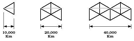
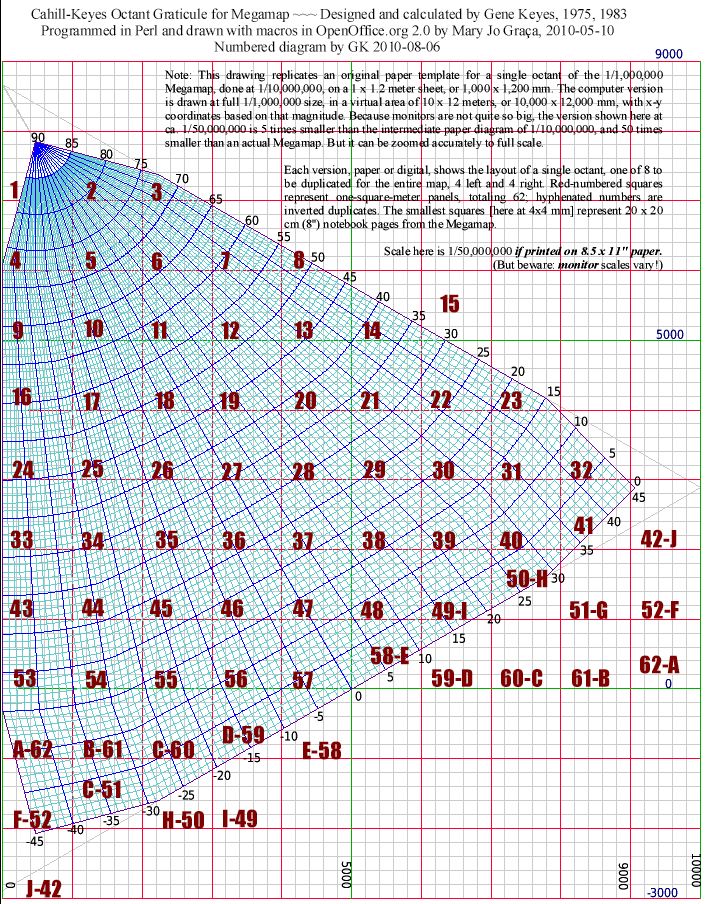
If you are doing this map in a vector-draw or CAD program, then one size fits all, depending on how big your monitor is, and how much you can zoom in or out. But in 1980, when I began hand-drafting the 1/1,000,000 megamap on separate square-meters of millimeter-grid cross-section paper, I compiled tables that were adaptable two ways: 1) for a single octant template (upright and tilted 30° to the left.) at 1/10,000,000, in a grid of 1,000 x 1,200 millimeters; i.e., just over one square-meter; 2) and for the scaled up Megamap itself, whose single-octant template would occupy 62 square meter sheets within a grid of 10,000 x 12,000 millimeters: (See diagrams below, and Photos of the Cahill-Keyes Megamap Prototypes.) That in turn is the prelude to a hoped-for 20 x 40 meter exhibition piece (65 x 130'). Therefore, numbers in tables 1 and 2 below on this page (for the hand-drawn version) are stated as coordinates of a millimeter grid that is 10,000 x 12,000 mm for the 62-sheet 1/1,000,000 template. (Note that x-line 0 starts 3,000 mm above the bottom of the grid, so as to intersect point G, which is the octant's central meridian, at the Equator's midpoint.) When I was simultaneously drafting the ten-times-smaller octant at 1/10,000,000, I would move the decimal one place to the left; i.e., I would read only the first column, [before the (*) digit]. (That would still yield a pretty big wall map, 2 meters high by 4 meters long, if the octant template is reproduced eight times.) The "Panel" column in table 1 refers to coding for the 62-square-meter version, shown as dark red numbers in Fig. 3 below. There are ten inverted-duplicate panels, to which I have appended letters A through J, in front or back, depending on whether they belong to the "up" or "down" portion of the wedges GHIJ or GHQR. (That latter "reciprocal wedge" GHQR is seen in Fig. 2, but not in Fig. 3.) 4) Orientation, computer-drawn
To repeat, these diagrams here on p. 1 show how I constructed one complete octant on paper, the 1/10,000,000 version, upright and tilted left. The specifications and tables on this page establish the basic shape, orientation and segment lengths of the complete Cahill-Keyes Octant Graticule. However, when it came to doing the same thing with Perl and computer graphics, Mary Jo's approach was to draft only half of an octant, lying horizontally, then copy, flip, and rotate it successively, via macros, to attain a full octant and then the complete eight-octant M-profile in its 40,000 km (mm) grid. Much easier said then done; but she did it, on her little Asus netbook. The specifications on pages 2 and 3 describe the exact graticule of a one-half octant, to be replicated 16 times (8 left, 8 right) for a complete world map. The macros shown on pages 4 and 5 draw that graticule. Though her coordinates occupy a lengthy and unabridged table for every single geocell, there are only half as many as in my original set. Despite her different orientation, the outcome is still the same eight-octant graticule for a 1/1,000,000 Cahill-Keyes Megamap — or any other specified scale or size. My hope is that it can then absorb all kinds of global data, and be useful to anyone who cares to work with it — in hard copy, or digital display, or both. (A related wish of mine is for counterpart one-degree and five degree globes, from small to giant, marked with the Cahill-Keyes octant. See FDR globe, etc., here, esp. figs. 9.6.6 and 9.6.12.) |
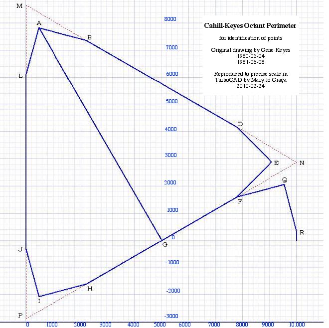
| Fig. 2: Cahill-Keyes Octant Perimeter
points. (Note that unlike an earlier version of this on my "Scaling..." page, midpoints
"C" and "K" are no longer needed. Also, point "G" is now set on the
zero y-axis, rather than y 200 as before.)
|
|
|
| 5) Coordinates for hand-drawn
version of octant perimeter
Deferring to Mary Jo's automated re-orientation
of the graticule's x-y coordinates (p. 2 and 3 below), I have omitted
most of my original whole-octant tables — except the ones given here, which
specify the original design framework and segment lengths (as shown above).
They remain the same in the subsequent computer-drafted version.
For a 1/10,000,000 map, read first column of digits only. For a 1/1,000,000 map, append (*) column's digit. Other decimals are for optional precision: e.g., if a 1/100,000 map, append first digit from four-place decimal column; for a 1/10,000 map, append the second; etc. Decimal places are for more exact computation, not visible to naked eye, until they start to cumulate. |
| Point |
Panel |
X |
* |
decimal |
Y |
* |
decimal |
|
| Scaffold
Triangle |
||||||||
| Base midpoint (altitude foot) |
G |
57 |
0500 |
0 |
0000 |
0 |
||
| Vertexes: |
||||||||
| M |
n.a. |
0 |
866 |
0 |
2541 |
|||
| N |
42-J |
1000 |
0 |
0000 |
0288 |
6 |
7513 |
|
| P |
J-42 |
0 |
-0288 |
6 |
7513 |
|||
| Octant
Perimeter Itself |
||||||||
| Vertexes |
||||||||
| Starting
point |
A |
1 |
0047 |
0 |
0000 |
0784 |
6 |
1902 |
| E |
42-J |
0906 |
0 |
0000 |
0288 |
6 |
7513 |
|
| I |
J-42 |
0047 |
0 |
0000 |
-0207 |
2 |
6873 |
|
| Q |
42-J |
0953 |
0 |
0000 |
0207 |
2 |
6875 |
|
| Joints |
||||||||
| B |
3 |
0222 |
4 |
0639 |
0737 |
6 |
1902 |
|
| D |
23 |
0777 |
5 |
9361 |
0417 |
0 |
8152 |
|
| F |
50-H |
0777 |
5 |
9361 |
0160 |
2 |
6875 |
|
| H |
H-50 |
0222 |
4 |
0639 |
-0160 |
2 |
6875 |
|
| J |
A-62 |
0 |
-0031 |
8 |
6236 |
|||
| L |
4 |
0 |
0609 |
2 |
1263 |
|||
| R |
62-A |
1000 |
0 |
0000 |
0031 |
8 |
6326 |
|
| Segment
Lengths, in mm |
mm |
* |
decimal |
|||||
Scaffold Triangle |
||||||||
| MN,
etc.: sides |
1154 |
7 |
0053 |
|||||
| MG,
etc.: altitude(s) |
1000 |
0 |
0000 |
|||||
| MB,
DN, etc.: vertex sides |
256 |
8 |
1278 |
|||||
| EN,
etc.: altitude indent |
94 |
0 |
0000 |
|||||
| MD,
etc.: vertex to 2nd indent |
897 |
8 |
8773 |
|||||
Octant Perimeter Itself |
||||||||
| AG
etc.: internal altitude |
906 |
0 |
0000 |
|||||
| AB,
etc.: each end-segment |
181 |
5 |
9406 |
|||||
| BD,
etc.: each mid-segment |
641 |
0 |
7498 |
|||||
| ABCDE,
etc. each 3-segment side |
1004 |
2 |
6307 |
| 6) Constructing meridians and parallels
in the Cahill-Keyes Octant Graticule (These specifications apply both to hand drawn and computer-drawn versions) Meridians Except where noted, parallels are mainly a
function of equisecting the meridians, so we begin with meridians.
Note: Below are construction numbers
for meridians in an octant, not their actual globe numbers, which are compiled
in a separate table.
M 0 [meridian zero, the central one] is the altitude AG, and is straight; all the others have two joints.Latitude lengths are the same for each respective plus-or-minus-numbered meridian, (e.g., anything on meridian 37 equals meridian (-37)., but they will have different x-y coordinates, as well as a specified variance (from earth itself) for each separate meridian pair-per-octant.. (All terrestrial degrees of latitude are ca. 111.111 km, but on this flat map, shrinkage is proportionally shared toward the octant's center, as adapted from Buckminster Fuller's Dymaxion map. Also, some other tweaks are made in the "supple zones" explained below.) Meridians are constructed in three zones:
Polar (ALB in diagram above),All meridian angles change from one meridian to the next at a constant rate: In the Polar zone, each meridian's angle is 1° greater or less than its neighbor, within a 90° spread. The three swathes of meridians bend at respective
joints which are not tangent to a parallel. [My earliest design bent
meridians from given parallels of 73° and 17°, but this resulted in disparate
meridian angles, and longitude widths, throughout.]
Parallels
Parallels, too, are constructed in the same three zones: 1) Polar, P 89 to 75: has concentric circular
arcs centered at the pole, A, with radii cumulating at 104 mm per degree
of latitude (104, 208, 312 mm etc.)
1a) Between M 30 and M 45 there is a polar "supple zone" (illustrated and further explained below). P 74 and 73 are circular arcs, but their radius increases by 100 mm per degree, instead of 104 mm. As well, P 74 and 73 are circular arcs only from M 0 to M 30. 2) The predominant Middle-sector,
P 73 to P 15, is where all meridians are equisected, and those points
are joined to form gradually flattening curves as they approach the Equator.
Here, all latitude lengths along the outer meridians (M 45) are 110.4278
mm. Along M 0, they are all 100 mm, and all meridians in between are
interpolated proportionately.
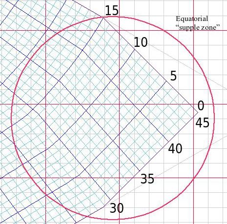
3) The Equatorial zone, P 15 to 0, is
where meridians are equisected with the same latitude lengths as above,
but only as far as M 30 on either side.
3a) Another “supple zone” is in the equatorial right-angle corners of the octant (Likewise illustrated and further explained below). It is an area comprising 15° each of latitude and longitude (M 30 to 45. and P 15 to 0), where the equisection is redistributed proportionately beginning from a longer latitude length along M 45: 121.0627 mm per degree instead of 110.4278 mm as in the Middle-sector. 7) Further explanation of the "supple zones"
To attain smooth continuity of parallels
across octants in the predominant Middle-sector, avoiding cusps and
sags, the Cahill-Keyes graticule adds a little extra stretch along the
outer edge (M 45), at two relatively small "supple
zones" (on each side of the octant, or four in all). The supple zones'
excess decreases evenly within the longitudes of M 45 to 30, between
the latitudes of P 75 to 73, and likewise within M 45 to 30 between P
15 to 0 respectively. The stretching is compensated by a small reduction
on M 45 in each Middle sector geocell height to 110.4078 mm, instead of
an ideal 111.1111, along M 45.
Polar supple zone:
Fig. 4: Diagram by Gene Keyes in
OpenOffice.org Draw 2.0; coding by Mary Jo Graça.
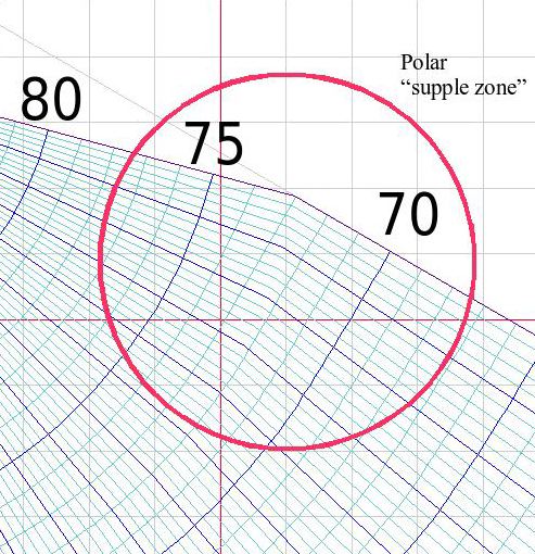
Fig. 5: Diagram by Gene Keyes in
OpenOffice.org Draw 2.0; coding by Mary Jo Graça.
|
| 8) Latitude lengths per 1 and 5 degrees
(These specifications apply both to hand drawn and computer-drawn
versions)in Cahill-Keyes Octant Graticule (central and outer meridians) For a 1/10,000,000 map, read first column of digits only. For a 1/1,000,000 map, append (*) column's digit. Other decimals are for optional precision: e.g., if a 1/100,000 map, append first digit from four-place decimal column; for a 1/10,000 map, append the second; etc. Decimal places are for more exact computation, not visible to naked eye, until they start to cumulate. |
| mm |
* |
decimal |
||||||
| 1-degree
Latitude lengths along M-0 |
||||||||
| P-90
to P-75 |
10 |
4 |
0000 |
|||||
| P-75
to P-0 |
10 |
0 |
0000 |
|||||
| 1-degree
Latitude lengths along M-45 |
||||||||
| P-90
to P-75 |
10 |
4 |
0000 |
|||||
| supple
zone P-75 to P-74 |
13 |
0 |
9883 |
|||||
| " P-74 to joint |
12 |
4 |
9523 |
|||||
| " joint
to P-73 (These 2 combined are also 130.9883) |
6 |
0360 |
||||||
| P-73
to P-15 |
11 |
0 |
4278 |
|||||
| supple
zone P-15 to P-0 |
12 |
1 |
0627 |
| 5-degree
cumulative lengths from pole onward |
M-45
mm |
* |
decimal |
M-0 mm
|
* |
decimal |
||
| 90-85 |
52 |
0 |
0000 |
52 |
0 |
0000 |
||
| 85-80 |
104 |
0 |
0000 |
104 |
0 |
0000 |
||
| 80-75 |
156 |
0 |
0000 |
156 |
0 |
0000 |
||
| [supple
zone, 75° to 73°] |
||||||||
| 75-74 |
169 |
0 |
9883 |
na |
||||
| 74-73
(as far as joint) |
181 |
5 |
9406 |
na |
||||
| P-74-73
(beyond joint |
181 |
9 |
9766 |
na |
||||
| 75-70 (including supple zone & joint) |
215 |
3 |
2600 |
206 |
0 |
0000 |
||
| 70-65 |
270 |
5 |
3990 |
256 |
0 |
0000 |
||
| 65-60 |
325 |
7 |
5380 |
306 |
0 |
0000 |
||
| 60-55 |
380 |
9 |
0770 |
356 |
0 |
0000 |
||
| 55-50 |
436 |
1 |
8160 |
406 |
0 |
0000 |
||
| 50-45 |
491 |
3 |
9550 |
456 |
0 |
0000 |
||
| 45-40 |
546 |
6 |
0940 |
506 |
0 |
0000 |
||
| 40-35 |
601 |
8 |
2330 |
556 |
0 |
0000 |
||
| 35-30 |
657 |
0 |
3720 |
606 |
0 |
0000 |
||
| 30-25 |
712 |
2 |
5110 |
656 |
0 |
0000 |
||
| 25-20 |
767 |
4 |
6500 |
706 |
0 |
0000 |
||
| 20-15 |
822 |
6 |
7890 |
756 |
0 |
0000 |
||
| Equatorial
zone with adjustments |
||||||||
| 15-10 |
878 |
5 |
9785 |
806 |
0 |
0000 |
||
| 10-5 |
941 |
4 |
3535 |
856 |
0 |
0000 |
||
| 5-0 |
1004 |
2 |
7285 |
906 |
0 |
0000 |
5-degree cumulative lengths from equator onward: equatorial segment only, P-0 to P-15 |
M-45 mm
|
* |
decimal |
M-0 mm
|
* |
decimal |
||
| 0-5 |
62 |
8 |
3750 |
50 |
0 |
0000 |
||
| 5-10 |
125 |
6 |
7500 |
100 |
0 |
0000 |
||
| 10-15 |
181 |
5 |
9395 |
150 |
0 |
0000 |
||
| M-45 5-degree re-cumulating lengths for Middle-Sector only from P-15 to P-73 |
||||||||
| 15-20 |
55 |
2 |
1390 |
50 |
0 |
0000 |
||
| 20-25 |
110 |
4 |
2780 |
100 |
0 |
0000 |
||
| 25-30 |
165 |
6 |
4170 |
150 |
0 |
0000 |
||
| 30-35 |
220 |
8 |
5560 |
200 |
0 |
0000 |
||
| 35-40 |
276 |
0 |
6950 |
250 |
0 |
0000 |
||
| 40-45 |
331 |
2 |
8340 |
300 |
0 |
0000 |
||
| 45-50 |
386 |
4 | 9730 |
350 |
0 |
0000 |
||
| 50-55 |
441 |
7 |
1120 |
400 |
0 |
0000 |
||
| 55-60 |
496 |
9 |
2510 |
450 |
0 |
0000 |
||
| 60-65 |
552 |
1 |
3900 |
500 |
0 |
0000 |
||
| 65-70 |
607 |
3 |
5290 |
550 |
0 |
0000 |
||
| supple
zone @ 1° |
||||||||
| 70-71 |
618 |
3 |
9568 |
560 |
0 |
0000 |
||
| 71-72 |
629 |
4 |
3846 |
570 |
0 |
0000 |
||
| 72-73 |
640 |
4 |
8124 |
580 |
0 |
0000 |