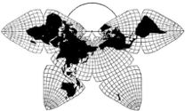
Cahill 1909
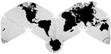
Cahill-Keyes 1975
|
Cahill 1909
|
Go back to
Gene Keyes home page
Cahill-Keyes 1975 |
|
Why Cahill? What about Buckminster Fuller?
Evolution of the Dymaxion Map: An Illustrated Tour and Critique Part 8 by Gene Keyes 2009-06-15 Summary: I
love Bucky, but Cahill's map is a lot better. Here's how.
CONTENTS Click inside boxes to open other sections in separate windows. |
|
Part 8
Notes on Scaling Dymaxion Maps As stated in my counterpart article to this,
I found various Cahill maps hard to scale, until I determined
that the span of an arch of 4 of its octants can be equivalent to half
a great circle, i.e., 20,000 km, and that 8 octants in my M-profile
represent 40,000 km, the earth's circumference. From this it is easy
to designate a standardized comparison scale of a Cahill or Cahill-Keyes
map in relation to a cognate globe, irrespective of compressions
or expansions within each octant, or other criteria being used.
Cahill-Keyes maps (but not Cahill) adapt the Fuller projection principle of having the outer edge of each flat facet be the same as its spherical counterpart. Moreover, each side of a Cahill-Keyes octant equals the original metric-system length of 10,000 km each (a meter being 1/10,000 the length from pole to equator). Thus any Cahill-Keyes map is easy to scale (and enlarge or reduce), given its outer-edge metric length of 10,000 km, and a rectangular span of 20,000 km per sub-assembly of 4 octants, or 40,000 km for all eight octants: an equatorial scale, as well as a pole-to-pole scale, as well as a global scale.. (See example here.) However, Fuller's icosahedrals are more difficult
to scale to a standardized number, or to an equatorial scale,
especially given the eccentric placement of its triangles vis
a vis the poles and equator. (An ordinary [Fisher] gnomonic icosahedral
map with vertexes at the poles, has a straight equator that is
easy to measure, traversing half the triangles — ten — at midpoint;
but they lack Fuller's achievement of unbroken continents, and unbroken
polar regions, especially the north pole. See appendix below.)
Meanwhile, Fuller's maps are labeled with a rubber scale, such as the original Dymaxion's "1/34,200,000 to 1/51,500,000", or, "1/47,500,000 to 1/57,000 000" on the Honeywell wall map (and mis-labeled on the much smaller Honeywell fold-up icosahedron because it was simply copied from a larger-scale wall map.) Which is the real scale? What this variability means is that the larger scale (i.e., the smaller-denominator fraction) is at the edges of a facet, and the smaller scales reflect the shrinkage toward the center of each facet. My Cahill-Keyes maps likewise shrink toward the center; but the comprehensive scale which I declare for them is both an equatorial scale, and based on one-quarter of a great circle, pole-to-equator. So taking the equator, and the two bounding meridians of each octant, just as they are seen on a globe, we have at one grasp the identical scale of the equator, and of the two defining great circle meridians transitting the poles, and of the equivalent globe. This cannot be said of any Dymaxion map, cubo-octahedral, or icosahedral, which, using those three approaches to assess its scale — equatorial; or pole-to-pole; or cognate globe — , yields three different results. 1) Equatorial? Hardly. On Fuller's first cubo-octahedron, the Equator was the diagonal of the four non-polar squares, and those diagonals in principle were each 1/4 of a great circle, i.e., 10,000 km; But because the Equator was not a facet edge, it goes through the shrink zone, and is actually 37,715.4 km. (See appendix below.) And the icosahedral is worse, equatorially. For instance, doing a quick rough measurement of equator lengths on the folding Honeywell edition of Fuller's icosahedron — the one with the wrong scale imprinted — , I found it traversed eight triangles, rather than ten (as in Fisher's), with lengths, in millimeters, of 80, 83, 20, 60, 77, 83, 23, and 60; and some of these lines were bent, rather than straight. Total equatorial length, 486 mm; divided into earth circumference of 40,000 km indicates an equatorial scale of: 1/82,000,000.
(As shown in #3 below, the equatorial length according
to the edge scale should be 516 mm, not 486.)2) Pole-to-pole? This thought occurred to me, because I noticed that on Fuller's laid-out icosahedral, it so happens that the 20,000 km distance between poles (assuming they are shown, on a given scale-less map), is half the left-to-right length of the upper five edges of the central keel comprising nine and a half triangles, which therefore would be equivalent to 40,000 km. A triangle edge of that folding icosahedron is 91 mm; × 5 = 455 mm, divided into 40,000 km, for a pole-to-pole scale of: 1/88,000,000
However, the actual km length of the 5
upper triangles is not 40,000, but only 35,244: see #3 just below. In fact,
it takes 5 and 2/3 triangle lengths to equal 40,000. Thus the pole-to-pole
and upper-edge equivalence is misleading, because, like the Equator, the
polar great circle has been variably compacted through six different graticules
of six triangles (and not eight like the Equator.) It is one more symptom
of what I regard as one of the Dymaxion maps' worst flaws, their totally
different graticules for each facet, unlike Cahill's identical graticules
in each octant.
3) Cognate globe, i.e., outer edges of each triangle? This one should be the clincher, because that is the true scale in any Dymaxion-projection map. Easier said than done. What is the terrestrial length of an icosahedral arc on a globe? Here is where:the icosahedron is much more difficult to scale and relate to a globe (despite nifty graphics of a globe becoming an icosahedron, then unfolding — see Part 7). An icosahedron, instead of having 90° edges like an octahedron, i.e., one quarter of a great circle, i.e., 10,000 km, has edges that are, as Fuller states in his broadsheet (Part 5 above), "63°, 26', 05.816 . . . . . . . " How much is that in kilometers? We shall see. Fuller's Dymaxion maps are very anti-metric, to say the least: He avoids their metric values as habitually as an American grocery store. (I speak as an American in Canada, a country whose grocery stores are at least half-heartedly metric.) What Bucky's icosahedrals also state is their triangle edge length in nautical miles. 3,806 nautical miles.
And what is that in kilometers? 1 nautical mile = 1.85200 km; thus: 7,048.712 km, per edge:
a very irrational non-metric amount, given that the entire basis of the metric System, the meter, in principle is 1 / 10,000 the distance from equator to pole.(Recalling that the correct-scale edge of any side of any Cahill-Keyes facet is 10,000 km.) As for the cubo-octahedron, Fuller had stated its edge-length, square or triangle, as 60º, or 3,600 nautical miles: × 1.85200 = 6,667.2 km per edge. But wait: in 1980, a more precise draft of a Fuller icosahedral was produced by Rob Grip and Chris Kitrick, with more decimal places: the icosa edge is now stated to be 63°, 26', 6.81576'', and the nautical miles are given as 3,806.09693: which gives us a new kilometer datum of: 7,048.891514 km, per edge.
Let's just call it 7,048.89 km. So therefore, instead of working with 10, or 20, or 40 thousand kilometers as quarter, half, or full great circle portions of the earth's circumference, we must divide a length in mm, of an icosahedral triangle side into that irrational 7,048.89. In the case of the foldup icosahedron, with 91 mm edges, divided into 7,048.89 we now get a (rounded) scale of: 1/77,500,000
I therefore declare that figure as the deciding scale, the principal scale, the best-out-of-three. It happens to be the largest because by definition, the Dymaxion projection is accurate on the outer edges of a facet, and compressed toward the middle. Ergo, any meridian or parallel, including the equator, is refracted through a large number of variable lengths, because no triangle on Fuller's icosahedron has a comparable graticule. (All octants in a Cahill map have identical graticules.) In fact, no meridian or parallel on a Fuller isosahedron is consistent or accurate compared to a globe. It is only the icosahedron edges which bear true allegiance, and none of them track a meridian or parallel. (On Cahill-Keyes, the equator and two principal meridians are equal to their global parent.)Consequently, Fuller's icosahedrals likewise downplay their graticule, either omitting it, or showing a widely-spaced 15 degree version, which I regard as almost useless. (In my "Geocells" paper, I mention that the exception is the Grip-Kitrick Fuller map, which has an over-cluttered and equally unreadable and unlabeled 1/2-degree graticule. (This point is illustrated and elaborated in Part 9.2.) As shown, Fuller did have a 5-degree graticule in the original Dymaxion cubo-octahedron. When he switched to the off-center but full-continent cubo-octahedron, the graticule got skewed and splayed and therefore was considerably de-emphasized, to 15°. The zig-zagginess of Fuller's folded icosahedron as compared to Cahill's folded polyhedron or flattened rubber ball, makes Fuller's much harder to grasp, at least for me. Fuller's equator meanders up and down; his off-center poles produce irregular deformed Arctic and Antarctic "not-circles". Cahill's equator is along the edges; his poles are at vertex antipodes of the top and bottom facets. To be sure, in devising the Dymaxion map, Fuller was also working out a new grid of great circles, and "Energetic-Synergetic Geometry", which led to the invention of the geodesic dome, but that is a different story. And I will concede this for a Dymaxion icosahedral: because there are more triangles, 20, than the 8 of an octahedral, there is less compressive distortion, per facet, in the icosahedral. But as I have argued throughout this presentation, the other distortions and overall design flaws of Fuller's icosahedral are so great compared to Cahill's octahedral, that I have long since opted for Cahill's. After all this roundabout, I now have the formulas to either find the scale of a Dymaxion map which lacks one, or to enlarge or reduce an image to fit a desired scale: Scale in millions to 1 = 7,048.89 km / edge in mm (icosahedron)
or 6,667.2 km / edge in mm (cubo-octahedron)
Edge in mm = 7,048.89 km / scale in millions to 1 (icosahedron) or 6,667.2 km / scale in millions
to 1 (cubo-octahedron)
That is, if I know the millimeter length of a triangle edge for the preferred scale, and I divide it by the millimeter length of an image on hand, I get the percentage to which I can raise or lower the map, using simple image software on a computer. (E.g., on my venerable Mac G3 OS 9, I have long used two pieces of invaluable freeware: Goldberg, and BigPicture 4.2. I could never have done all this so easily back in 1969-1975, when I was first examining the Dymaxion Map in minute detail.) For example, what is the icosa-triangle edge length in millimeters of a 1/100,000,000 map? Now it's easier: divide 7,048.89 by 100, and we get 70.5 mm. Ditto for a 1/200,000,000 map: divide 7,048.89 by 200, and get 35.2 mm. Suppose we have a map with edges of 91 mm, and want to enlarge it to 1/50,000,000: whose edges would be 141 mm: Divide 141 by 91, and get 154.9%. So one enters 154.9% in the image-handling software. Or, if we had already figured that the 91-mm-edge map is 1/77,500,000, then we could divide 77.5 by 50, and get 155%, close enough Similarly, if we want to reduce that 1/77,500,000 map to 1/100,000, we can either divide their edge lengths 70.5 / 91 = 77.5%; or, divide 77.5 / 100, and sure enough, get 77.5%. PS: as I point out elsewhere, lengths will vary according to your computer and monitor and resolution; therefore, these formulas apply in the first instance to print versions of maps; and you will have to make your own adjustments, if your results are different when you hold a ruler up to your monitor. (Even when I have drafted maps on millimeter-grid paper, I found that different rolls of K&E paper might not be 100% congruent. And different millimeter rulers did not always agree with each other. To say nothing about humidity. Or relativity.) Appendix
Further remarks on the compressive effect
of the Dymaxion Projection
(and my adaptation of it) Where the elasticity is a problem is the fact that when a spherical triangle is flattened from its outer edges inward, its internal altitude becomes shorter than its outer sides. (On an octahedral sphere, altitude and sides are all equal, each of them being 1/4 of a meridian, or equator. On a Cahill-Keyes map, the equator and outer meridians are true to scale, but the altitude meridian has the most compression.) Therefore, if the flat-triangle internal altitude is to scale with its corresponding globe, then all the outer sides are too large. Or, if the outer sides of the triangle are to the same scale as that globe (in the Fuller and Cahill-Keyes transformations), then the inner meridians and parallels are progressively too short. One way to see the internal shrinkage is to notice that on the original 1943 cubo-octahedron, the Equator is the diagonal of the four squares, which should equal 40,000 km. However, doing some simple calculator math for a hypotenuse length shows that the 1943 Dymaxion map Equator is only 37,715.4 km, or a 5.7% dimunition: thus Edge length of square, as stated by Fuller: 3,600 nautical milesAlternately, one can simply measure the square facets as printed in the Life center-spread: Square edge, 156 mm; its km length, 6667.2; ÷ 156 = 1/42,700,000 as already derived for principal scale of that cubo-octahedron. * (Oops: in the Life Magazine cut-out print, the Scale legend on the map [Argentina triangle: see Part 2, Fig. 2.18] says that the "diagonals of squares are 5400 nautical miles, 1/4 of a Great Circle, 90 degrees". Not quite! Of course, Fuller can state the diagonals to be 5,400 nautical miles instead of 5,091; but then the outer edges would be correspondingly larger, and therefore not a true Dymaxion map with edges in scale to a globe. Indeed, the 4 non-polar diagonals on the 1943 Dymaxion map do track the Equator, and represent its 14,400 nautical miles — but not at the same scale as the facet edges!) Therefore, one cannot ascertain the principal scale of a 1943 Dymaxion along the Equator. As with the 1954 icosahedron, scale must be measured on the outer edge of the facets. (The cubo-octahedron has the same length for triangles or squares). Perhaps at this point I should state a principle: when I say "principal scale" regarding a map such as Fuller's Dymaxion, or the Cahill-Keyes adaptation of it, then I am referring to the declared true scale of the outer edges of a facet. We disregard the progressively smaller scales toward the interior of each facet, in favor of taking the map as a whole in relation to its cognate globe. An alternate nomenclature might be "global-cognate scale".The principle is that the edge scale matches the cognate globe. This makes it the principal (and largest) among various scales to be found in a Dymaxion (or Cahill-Keyes) polyhedral map. Either spelling of the word is correct. |
| Fig. 8.1 below: A similar disparity can
also be seen on a non-Fuller gnomonic icosahedran a la Fisher (below)
aligned to the equator and poles. The equator is a straight line
bisecting the central keel of ten triangles (five pairs of two),
and exactly the same length as the five upper or lower edges of that
set. However, the otherwise globally identical north-south
great circle only traverses a row of eight triangles (four pairs
of two, not five pairs of two).*
In the first image, I have adjusted the equator
to be 200 mm long, for an (equatorial) scale of 1/200,000,000.
[On my monitor.] But measuring from pole to pole (times
two), and perpendicularly, not diagonally, we find a bigger total length
of 222 mm, or 1/180,000,000. Since the equator occurs at midpoint of
its respective triangles, it has not been "blown up" as much at the
extremities, as with a gnomonic (or Mercator) projection.
*Discussion assumes perfect earth-sphere, not ultra-precise "spheroids". |
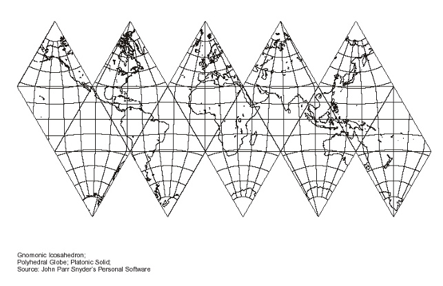
Source: Paul B. Anderson,
http://www.csiss.org/map-projections/Polyhedral_Globes/Icosahedron_Gnomonic.pdf
converted to jpg by Gene Keyes and size adjusted
to 200 mm equator.
|
| Fig. 8.2 below: So next we reduce the
up-down pole-to-pole length to 100 mm, which when doubled to
a full great circle, now makes the map 1/200,000,000 in relation
to its polar distance, but the equator has shrunk to 182 mm, for
a smaller equatorial scale of 1/220,000,000.
|
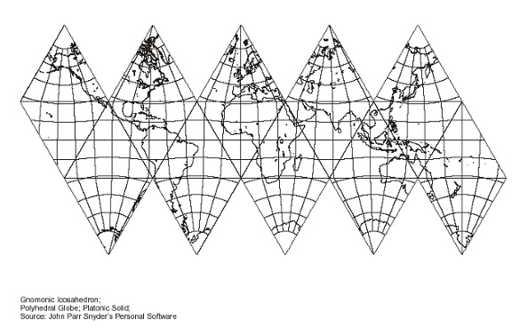
Source: Paul B. Anderson,
http://www.csiss.org/map-projections/Polyhedral_Globes/Icosahedron_Gnomonic.pdf converted to jpg by Gene Keyes and size reduced to
100 mm pole-to-pole distance.
|
| Fig. 8.3 below: In the next two
examples below, I am showing a Dymaxion icosahedron specimen by Robert
W. Gray: taken directly from the Web, at an unstated scale. First, using
the formulas explained above, we find a triangle length of 38.8 mm [on
my monitor; adjust your image if necessary]; divided into
7,048.89, for a main scale of 1/181,000,000. (Note: individual edge
lengths were measured in upper group of five, total length 194 mm; divided
by 5 = 38.8.)
|
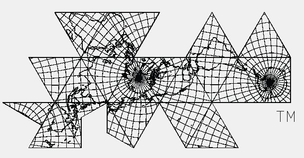
Source: Robert Gray, http://www.rwgrayprojects.com/rbfnotes/maps/images/fmap3.gif
converted to jpg by Gene Keyes |
| Fig. 8.4 below: Next, I reduce the map to 91.1%, for
a main scale (edge of 35.2 mm) of 1,200,000,000.
|
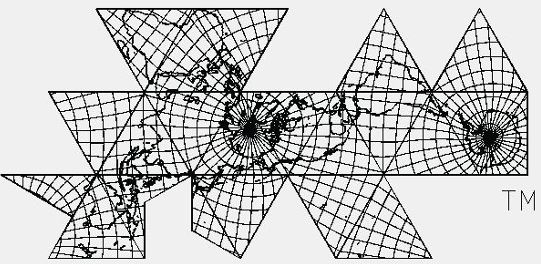
Source: Robert Gray, http://www.rwgrayprojects.com/rbfnotes/maps/images/fmap3.gif
converted to jpg and reduced to 91.1% by Gene Keyes |
| Fig. 8.5 below: Another example: here is
the Bank of Nova Scotia magnetic map, tweaked a bit to reduce it
to 1/200,000,000 from its original edge scale of 1/190,000,000.
|
Source: scanned by Gene Keyes from personal copy,
2007-04-07.
R. Buckminster Fuller and Shoji Sadao, Cartographers © 1954, 1972 by Buckminster Fuller (Full-size version in Part 6, Fig. 6.5.) |
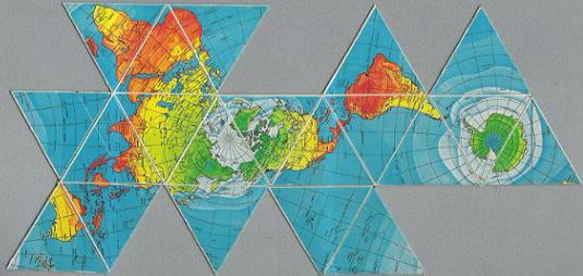
| Fig. 8.6 below: For scale comparison: a
Cahill N.Pacific-oriented Butterfly (1919), re-scaled to same as previous
two examples, 1/200,000,000. (Repeat of Fig. 9.1.1 in Part 9.1.)
|

Source: B.J.S. Cahill, "A Unique Commercial
Atlas and World Map" (Pacific Marine Review, [1920]-03)
p. 112. Scanned and digitally remastered with ClarisWorks 5 by Gene Keyes
from an illustration in a different layout in B.J.S. Cahill, "The
World Through German Goggles" (Pacific Marine Review, [ca.
1919-11]. Map enlarged to 208% of original. (Offprint quality of
latter better than Xerox of former.)
Note: All maps in my B.J.S. Cahill Gallery were also re-scaled, up or down, to 1/200,000,000. |
| Having shown the Dymaxion map in its various stages
since birth in March 1943, I turn now to the critique. If Fuller's map
had burst on the scene without Cahill's accomplishment, then the Dymaxion
would be a unique step forward in cartography. Instead, it was a big step
backward. Cahill with long intensive effort had already produced a polyhedral
portrait of earth with unbroken continents, in a design far superior to
Fuller's. (And a triad of variants besides, not discussed here.)
Despite Life's proclamation that the Dymaxion map "is Designed for Political Geographers", that is not the case. Fuller was avowedly anti-political. He saw his map as a harbinger of his massive theory of Energetic-Synergetic Geometry, not as a tool of political and historical geography for a political scientist like me. Cahill, on the other hand, had intended his map for an array of social studies, meteorology, "geosophical analysis", and any other use to which maps are commonly put. But he was blindsided by John Paul Goode, and posthumously upstaged by Buckminster Fuller. (To say nothing of Arno Peters.) That said, the Dymaxion map is a worthy artifact indeed, and worth examining and criticizing in detail. Without Cahill, it might stand unchallenged. But I argue that in the realm of world-map cartography, at least, Bucky Fuller is bested by B.J.S. Cahill. |