Cahill-Keyes Octant Graticule and Grid

Cahill-Keyes Octant Graticule:
Principles and Specifications

with Perl programs and OpenOffice.org 2.0 macros
for 1/1,000,000 Megamap

Gene Keyes
2010-08-20

14) Cahill-Keyes Octant Graticule
and Megamap Grid as
illustrated from OOo macros

Grid protocol in the Cahill-Keyes "Real-World" Map

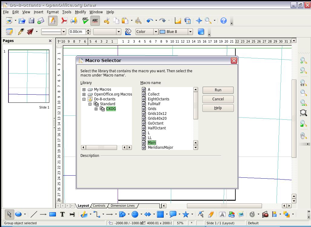
Among my Ten Principles for a Coherent World Map System is that the 1/1,000,000 Master World Profile, the Megamap, be inscribed exactly within a grid whose length is 40,000 mm [= km], representing the earth’s circumference. (The grid can be square, 40 x 40 m, or rectangular, 40 x 20 m; see Note below.) Mary Jo's macros integrate this grid principle with the Octant Graticule itself..

At any scale in the System, the map is shown within a specified progression of grid-squares. For instance, when the map is seen filling a notebook-size 8-inch square frame (200 x 200 mm), it is designated Scale 1, Size 1; its l-mm grid represents 200 km per mm; and the scale is 1/200,000,000. (This is the scale I used in my gallery of Cahill and similar maps.)

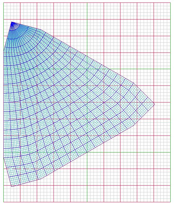
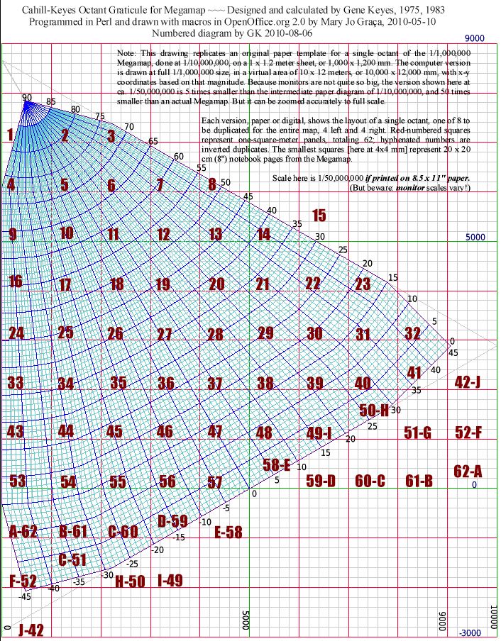
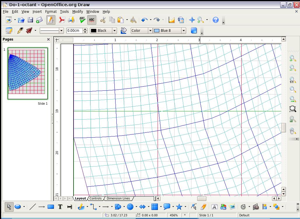
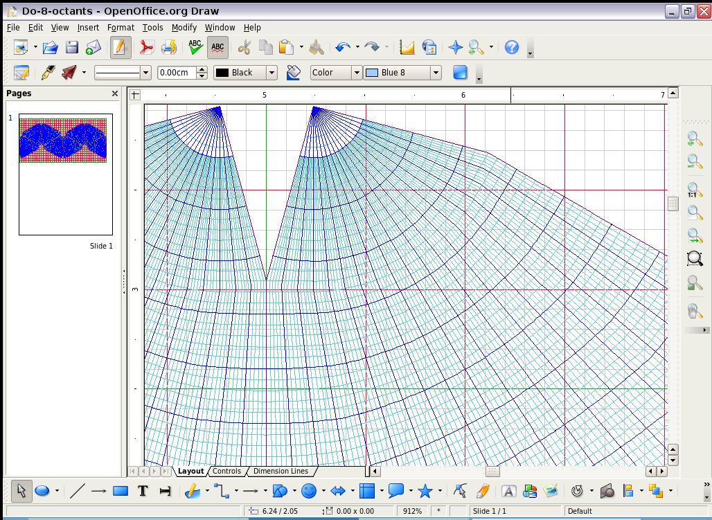
The entire kilometer grid is accented by three colors of sub-squares:

(1) the largest, with green lines comprising 5,000 x 5,000 km each; in turn divided by five for the next largest squares:

(2) with major lines in red comprising 1,000 x 1,000 km each, and then divided by 5 again for the smallest squares

(3) within the major ones, having light grey lines, 200 x 200 km each.

At 1/200,000,000, the smallest (light grey) square is 1 millimeter. At 1/1,000,000, the size of that smallest square (light grey) has dilated to 200 x 200 mm (= km), and could now show a new intervening grid of 1 mm, to represent 1 square kilometer each. As of this writing, the macros have not been extended to scales beyond 1/1,000,000, but the intent and principle is there, to do portions of the Cahill-Keyes map up to at least 1/5,000. (See "Ten Principles...")

In other words:

Until it reaches the scale of 1/1,000,000, the smallest (light grey line) squares in any Cahill-Keyes map represent 200 x 200 km.
The next larger accented squares, red-line, represent 1,000 x 1,000 km. (The red lines also represent the 1-square meter panels of the Megamap as diagrammed in Fig. 9 below and shown in the photos of the hand drawn test panels.)
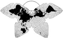
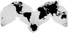
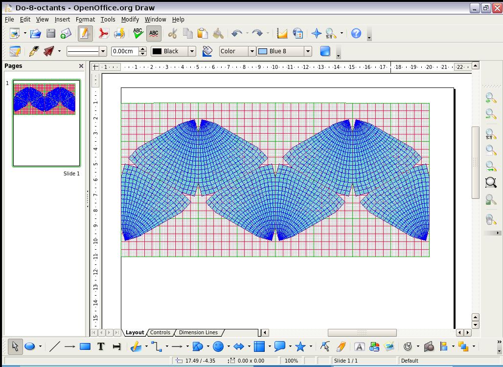
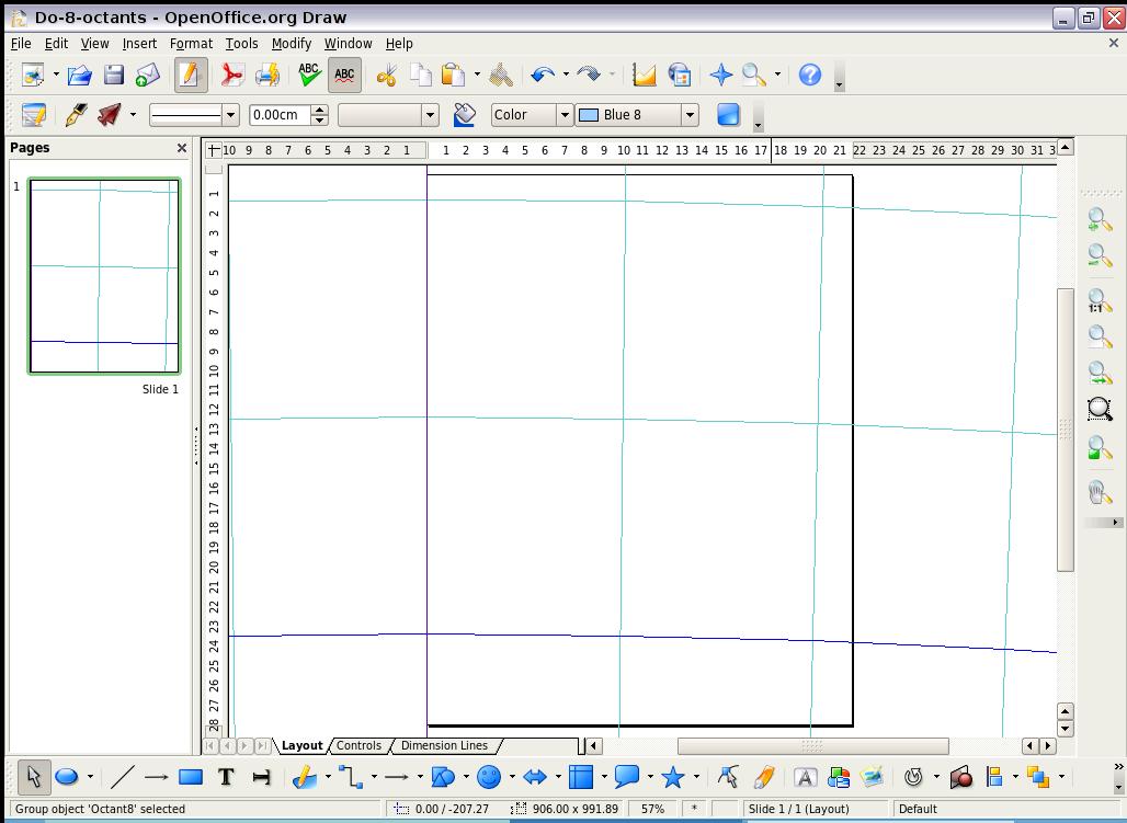
The largest accented sub-assembly of squares, marked with green lines, is 5,000 x 5,000 km, of which there are 4 x 4 per four-octant set, or 4 x 8 if in a rectangular frame for the full eight-octant world map, spanning 40,000 km, Q.E.D.

Note: A full 40 x 40 m square could have extra graphics such as counterpart global images, but where wall or floor space is limited, a 40 x 20 "double-square" frame includes the entire Cahill-Keyes map. Although the System is based on square frames, the third column in the table below shows the length of such rectangular "double squares" to accomodate the 40,000 km span of the M-shape Master Profile, and the last three columns show the length of sub-squares within the main frame.at specified scales.

Table 6: Dimensions of square (or rectangular) frame, and grid squares, for entire 8-octant Cahill-Keyes World Map, and their respective scales.

Below are shown some preliminary graphic outputs from the string of Perls and macros. I have already cautioned that your monitor may not show these in correct proportions. Sharpness is also a problem in the monitor (non-print) versions; see further comments below.

Fig. 7: This is the output of file "Do-1-octant.odg" showing both a whole octant, and its relation to the grid, all of whose squares expand or contract matching the scale of the map itself, and include the same array of meridians and parallels at any size. Note also that in this example, the green accent squares are "off center" because the zero y axis starts 3000 km above the bottom of the map, and because the drafting grid for a single octant and its scaffold triangle (seen in Fig. 9 below) is 10 x 12, not a square.

Fig. 8. Screenshot of in-progress "Do-8-octant" version, at 1/200,000,000. However, what you see on the screen here is 1/200,000,000 only if it is 200 mm (8") wide. Otherwise, it's a plus-or-minus thing.

Note that the macros produce a full 1/1,000,000 original, and then reduce it to any given scale: this one in principle being 200 times smaller. A unique fundamental of the Cahill-Keyes system is that it is always the same map at any size or scale, in whole or in part. Therefore, it is drafted in simultaneous versions from gym-size to notebook-size..

(Of course, content generalization, and lettering size, would have to be adjusted at given scale intervals. Perhaps this could be done as layers, not yet implemented in its present state of macro development.)

Sharpness is always a problem in these onscreen non-print versions. The screenshot below is only a jpeg. To see the one-degree geocells best at such a small scale, you should do a printout of this pdf (252 kb), exported from the map-image itself in Fig. 8 below, composed at 1/200,000,000. When the pdf is printed, even at the very small 8-inch-notebook-size scale of 1/200,000,000 the one-degree geocells, as well as the mm grid, are quite discernible!

Otherwise, if you open that pdf onscreen at 100%, the 3-color grid is hidden by the octants; But if you enlarge the pdf to 400% (1/50,000,000) onscreen, the relation of the grid to the octant-graticule is much more visible. Go to 1,000% in the pdf, and it is the scale of my prototype wall map, 1/20,000,000.

Fig. 9 Reprise of Fig. 3, p. 1, showing 3-color grid, scaffold triangle, and panel numbering,

Fig. 10 (reprise of Fig. 4, p. 1); showing grid at a larger scale. Note also the correlation between the size of the grey grid-squares (=200 x 200 km), and the one-degree geocells (= ±111 km of latitude each). Scale here is ca. 1/10,000,000 if grey squares are 20 mm.

I close with some screenshots of the macros at various stages as they draw the Cahill-Keyes Octant Graticule, in one and eight-octant versions. Note: Mary Jo and I both have Asus 701 eee netbooks (Linux-Xandros). She did all her work in the little netbook itself and its 7" screen, whereas mine is hooked to a 17" monitor, from which these shots are made.

Here in Fig. 11 is the result of step 2 in the macro sequence with file “Do-1-octant.odg”, where the octant has been drawn prior to the grid. Its perimeter is a purple line at the left (meridian -45). The vertical black rectangle represents a letter-size page. All that can fit in it are meridians -45, -44, and -43, and parallels 16 and 17. (Note that different printers have different margins, and no margins were set here. Also note that this is 57% of the full-size 1/1,000,000 map.)

Fig. 12: Here is the fifth step, after the grid has been added, and the octant moved to the front. Its purple perimeter line at the right covers the green outer grid line.

Fig. 13: Next we have a similar view as in Fig. 12 but now at 100%, a full 1/1,000,000 — except that I can't vouch for the size or accuracy of your monitor, nor mine. If the vertical green and grey lines are 200 mm apart, then the scale is right. Otherwise, only approximate. (Note: This is from step 3, before the octant was moved to the front, so in this case, the green outer grid line covers the purple perimeter line at the right.)

Fig. 14: If we zoom out to 20 times smaller, i.e., 1/20,000,000 (the scale of my hand drawn wall-map prototype), then we see where those two geocells fit (plus four truncated ones.). Scale again depends on your monitor. If the red squares were 100 mm on a side, we'd have 1/20,000,000. Otherwise, not quite . . .

Fig 15: However, this shot is a better approximation of 1/20,000,000: at least on my monitor, the grey squares are about 20 mm on a side, and the red squares, about 100 mm. In this case, I was re-zooming in from the whole-octant view in Fig. 7, instead of reducing, as in Fig. 14. Hopefully, future macros will enable more precise scale adjustments for difffering monitors, in addition to their existing precision when printed. (Note: Here again, the octant is in front of the grid, so its purple perimeter covers the green grid line — down to where the perimeter swings leftward. Then the green is visible again.)

Fig. 16: The last three screenshots are from the macro's eight-octant version. Here, step 2, the pre-grid plot of the octants, reduced onscreen to 57%.

Fig. 17: An example of the cumbersome dialog box to run the OOo macros.

Fig. 18: A parting shot. Notice once again, and in all other examples here, the foundation principle of the Cahill-Keyes Octant Graticule: namely, the proportional geocells: none severely different in dimension from any of its neighbors: whether single ones, or 5 x 5 groups. This aspect is what one sees in any large-scale regional map. But Cahill-Keyes is the first to show all geocells, proportional, in a single entire world map, at any scale from smallest to largest.

Now let globes show all one or five degree geocells, too. Their resemblance to a flat Cahill-Keyes "Real-World" map will be obvious.

Closing remarks

At this point, we have proof-of-concept that the Cahill-Keyes Octant Graticule can be drawn, with high precision,

using OOo macros
derived from a pair of Perl programs:

— all done by Mary Jo Graça on a $300 netbook with a free OpenOffice.org 2.0 vector draw program —

accurately, and
with one-degree geocells, and
as a single octant, or
as a complete 8-octant profile, and
at an original scale of 1/1,000,000 or any smaller ones,
(or larger, with additional tweaking),
in a grid whose squares represent 200 km, 1,000 km, and 5,000 km, and
exactly in a frame length representing 40,000 km, earth's circumference.

Next steps remaining include:

Easier method (buttons?) to change size and scale;
Repetitive numbering of all 1° parallels and meridians (at larger scales);
Repetitive numbering of all 5° parallels and meridians (at smaller scales);
Numbering of km spans across entire length of given map;
Numbering of all octants 1-8 (faintly);

and last but not least:

Incorporation of coastline and geopolitical data and the like.

System Scale #	Scale, RF	Square (or rectangle) length, mm	Green-line subdivision @ 5,000 km	Red-line subdivision @1,000 km	Grey-line subdivision @ 200 km
1	1/200,000,000	200	25 mm	5 mm	1 mm
2	1/100,000,000	400	50 mm	10 mm	2 mm
3	1/50,000,000	800	100 mm	20 mm	4 mm
		Square (or rectangle) length, meters
4	1/20,000,000	2	250 mm	50 mm	10 mm
5	1/10,000,000	4	500 mm	100 mm	20 mm
6	1/5,000,000	8	1,000 mm	200 mm	40 mm
7	1/2,000,000	20	2,500 mm	500 mm	100 mm
8	1/1,000,000	40	5,000 mm	1,000 mm	200 mm